Compile and run
In order to run the first example go into the ulambator folder and type `make tutorial1`. An executable will be created. Type `cd ..` and copy it to a work directory of your choice then type `./tutorial1.o` to execute the program.
Interface data ‘bnd0pos.dat’ and ‘ulamgeo2d000.vtk’ and velocity and pressure fields will be written in ‘ulam2d000.vtk’ and ‘ulamviz0.dat’. The VTK files can be used with ParaView and ‘bnd0pos.dat’ can be plotted with the Matlab code found in ‘tools/plot4ulambator.m’. The ‘ulamviz0.dat’ file can be visualized with ‘tools/ulamvisual.m’.
Also a ‘log0.txt’ file was created, which can be looked at with a text editor. It gives the system times for four instance: 1) at the beginning, 2) after solving the problem 3) after computing the matlab field data and 4) after computing the ParaView field data. This allows to get an idea of the computation times.
Tutorial 1 – Single phase flow in a bend
In this tutorial you will learn how to create fixed boundaries and to solve a single phase flow.
/* Ulambator configuration file Date: 09.12.2014 Version 0.7 */File Header
Together with included classes we add Ulambators matblc1.h and bndblock.h, which manage the geometry and generate the matrix that solves the posed problem.
#include "../source/matblc1.h" #include "../source/bndblock.h" #include <iostream> #include <stdio.h> #include <sys/time.h> #include <time.h> #include <math.h>The program begins with int main and prints a greeting to the screen.
int main (int argc, char * const argv[]) { std::cout <<"Welcome to ULAMBATOR++ v.7\n"; std::cout <<"Unsteady LAminar Microfluidic Boundary element Algorithm To Obtain Results\n"; char* savedir;Defining the geometry
The object bem is a boundary block, which works as a container that will manage all boundaries like fixed walls and liquid interfaces. Here we initialize the container to contain only a single boundary.
int number_of_boundaries = 1; BndBlock bem = BndBlock(number_of_boundaries);Two arrays are created. Position data of the boundaries in pos takes up to six values and boundary conditions bcs usually take two values.
double bcs[] = {1.0, 0.0}; double pos[6];The first boundary, boundary 0, is initialized (C++ starts counting from 0 unlike Matlab). The boundary will consist of 6 panels and the number of discrete elements num_elements per panel is 30 per unit length. The boundary is of type 0, type 0 means fixed boundary.
int num_panels = 6; int num_elements = 30; int type_boundary = 0; bem.Elements[0].Init(num_panels, 24*num_elements,type_boundary);The first panel of boundary 0 is initialized with num_elements elements and it belongs to geometry type 0, a straight panel. The boundary condition type is 3, a Poiseuille inflow boundary condition. The array bcs has no x and y velocity and the pos array contains the start point x,y and end point x,y coordinates.
pos[0] = 0.0; pos[1]= 1.0; pos[2]= 0.0; pos[3] = 0.0; int geo_type = 0; int bc_type = 3; bem.PanelInit(0,num_elements, geo_type, bc_type, bcs, pos);Panel 1. The boundary condition type is 0, a no-slip boundary condition. The last point of the former panel is the first point of the new panel.
pos[0] = 0.0; pos[1]= 0.0; pos[2]= 6.0; pos[3] = 0.0; bc_type = 0; bem.PanelInit(0,num_elements*6, geo_type, bc_type, bcs, pos);Panel 2, again with no-slip boundary condition.
pos[0] = 6.0; pos[1]= 0.0; pos[2]= 6.0; pos[3] = 6.0; bem.PanelInit(0,num_elements*6, geo_type, bc_type, bcs, pos);Panel 3, with constant normal pressure boundary condition.
pos[0] = 6.0; pos[1]= 6.0; pos[2]= 5.0; pos[3] = 6.0; bc_type = 2; bem.PanelInit(0,num_elements, geo_type, bc_type, bcs, pos);Panel 4, again with no-slip boundary condition.
pos[0] = 5.0; pos[1]= 6.0; pos[2]= 5.0; pos[3] = 1.0; bc_type = 0; bem.PanelInit(0,num_elements*5, geo_type, bc_type, bcs, pos);Panel 5, again with no-slip boundary condition.
pos[0] = 5.0; pos[1]= 1.0; pos[2]= 0.0; pos[3] = 1.0; bem.PanelInit(0,num_elements*5, geo_type, bc_type, bcs, pos);More information of different Panel types and boundary conditions is found in the Manual under PanelInit. Note that the variables can be overwritten hereafter since the information is passed on. One could also provide directly the numerical values to ‘PanelInit’, this rather explicit way was adopted to be more verbose.
Configuring the problem to solve.
At this point all boundaries and all panels are defined. This finishes the initilization of the BndBlock and we can create the matrix object. A matrix is created with the provided geometry bem, the aspect ratio LH, the viscosity ratio = zero and an unused number. A variable that represents the channel aspect ratio L/H, the non-dimensional channel height is 1/LH.
double LH = 8.0; MatBlC1 mat(&bem, LH, 0.0, 1.0);The directory savedir is passed to the matrix object (and automatically to the Bndblock). Make sure that the folder exists.
savedir = new char[120]; sprintf(savedir,"."); std::cout<<savedir<<"\n"<<std::flush; mat.EnableWrite(savedir);A log file log0.txt is prepared with a header, if the file exists it will be deleted. If you want to append data to an existing log file don’t call LogPrepare
mat.LogPrepare(0, "Computation time\n");Write all boundaries into the savedir (or subfolder) (here: bnd0pos.dat)
bem.allWrite();Save time step, time in the simulation and computation time to log0.txt
mat.LogRuntime(0);Build, Solve and visulaize the solution
Save the flowfield to a ParaView readible vtk file, this required to Build and Solve before. Build the matrix, provide a timestep for stabilization (set deltaT=0 for no stabilization). Then solve the matrix to obtain stresses and velocities. The file will be called ulam2d000.vtk, a unit length is discretized with 30 points and the visualized window ranges from x=0 to 6 and y=0 to 6.
mat.Build(0.0); mat.Solve(); mat.LogRuntime(0); mat.VisMatlab(0, 50, 0, 6, 0, 6); mat.LogRuntime(0); mat.VTKexport(0, 50, 0, 6, 0, 6);This provides a flowfield, normalization may be required
A last log of the time. Make sure all files are closed to avoid data loss.
mat.LogRuntime(0); mat.DisableWrite();End of program
std::cout << "Finished and Exiting\n"; return 0; }Result
When you run the file as it is you obtain an output that can be plotted in ParaView. Here we plot the pressure field from ‘ulam2d000.vtk’ and have ParaView compute the streamlines from the velocity field.
We use ‘ulamgeo2d000.vtk’ to plot the outer walls in black.
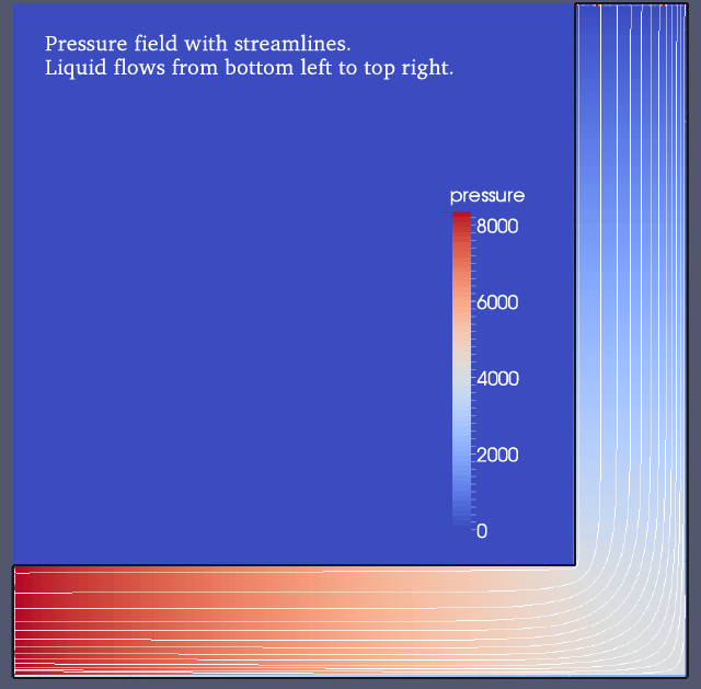
The pressure drops from about 8200 at the inlet to 0 at the outlet. An analytical result for the 2D Brinkman equation for straight channel flow at aspect ratio W/H=8 would have given 827.7 per unit length. The analytical result for the 3D Stokes equation in a straight channel would have given 833.7, quite similar. When counting only the two straight segments whose length is 5 the theoretical predicted pressure drop is in the order of 8300.
What would that be Pascals or bars? The dimension of the pressure is given as P = µ U/L. In this example we say the viscosity is that of water µ = 1 milli Pa s, the mean in flow velocity U = 5 mm/s and the channel width W = 96µm. Since the non-dimensional channel width is 1, the channel height is 12µm, which verifies W/H = 8. The aspect ratio and channel geometry was used in the numerical calculatio to obtain the non-dimensional pressure drop ∆p = -8200. ∆P = P*∆p = 0.0521*8200 Pa= 427 Pa or 4.27 milli bars.