Compile and run
In order to run the first example go into the ulambator folder and type `make tutorial2`. An executable will be created. Type `cd ..` and copy it to a work directory of your choice then type `./tutorial2.o` to execute the program.
Series of interface data ‘drop0tsnnn.dat’ and ‘ulamgeo2dnnn.vtk’ and velocity and pressure fields will be written in ‘ulam2dnnn.vtk’ or ‘ulamviznn.dat’. The VTK files can be used with ParaView and DAT files can be plotted with the Matlab.
This executable is configurable from the command line, type ‘./tutorial2.o 1 4 0.0’ and you will simulate a steady droplet in subfolder ‘test1’ with an aspect ration radius/channel height of 4 and zero eccentricity. When you measure the pressure inside the droplet you will see that it correponds to p=2*4+ π/4, which follows from Laplaces law. Where pi/4 comes from the in-plane curvature, which is 1 because the radius is 1 and pi/4 come from a correction by Park and Homsy (reference in our article) for flattened droplets. And where the out-of-plane curvature κ=2/h, here h = 1/4.
Tutorial 2 – Droplet relaxation
In this tutorial you will learn how to create a liquid interface and let it evolve in time. To this purpose an elliptical interface is created and a time marching follows the reaxation of the droplet.
/* Ulambator configuration file Date: 09.12.2014 Version 0.7 */File Header
Together with included classes we add Ulambators matblc1.h and bndblock.h, which manage the geometry and generate the matrix that solves the posed problem.
#include "../source/matblc1.h" #include "../source/bndblock.h" #include <iostream> #include <stdio.h> #include <stdlib.h> #include <sys/time.h> #include <time.h> #include <math.h>The program begins with int main and prints a greeting to the screen.
int main (int argc, char * const argv[]) { std::cout <<"Welcome to ULAMBATOR++ v.7\n"; std::cout <<"Unsteady LAminar Microfluidic Boundary element Algorithm To Obtain Results\n"; char* savedir;Defining the geometry
The object bem is a boundary block, which works as a container that will manage all boundaries like fixed walls and liquid interfaces. Here we initialize the container to contain only a single boundary.
int number_of_boundaries = 1; BndBlock bem = BndBlock(number_of_boundaries);We initilize three variables that allow parametrization from the command line. A variable that represents the channel aspect ratio L/H, the non-dimensional channel height is 1/LH. The eccentricity of the elliptical droplet and a folder identification number.
double LH = 8.0; double eccentricity = 0.95; int folderid = 0;Here the program catches the numbers that were passed when it was called eg. ./ulambator_main.o 1 5 0.5 sets the folderid=1, LH=5, eccentricity=0.5
if (argc>3) { folderid = atof(argv[1]); LH = atof(argv[2]); eccentricity = atof(argv[3]); }Output to the screen of the parameters.
std::cout<<"Elliptic Droplet Simulation, L/H "<<LH<<" eccentricity "<<eccentricity<<" folder no. "<<folderid<<".\n";Two arrays are created. Position data of the boundaries in pos takes up to six values and boundary conditions bcs usually take two values.
double bcs[] = {0.0, 0.0}; double pos[6];The first boundary, boundary 0, is initialized (C++ starts counting from 0 unlike Matlab). The boundary will consist of one single panel and the number of discrete elements num_elements is 300. We chose to reserve twice as much memory if due to deformation and remeshing the number of unknowns increases. The boundary is of type 2, type 2 means a droplet boundary.
int num_panels = 1; int num_elements = 300; int type_boundary = 2; bem.Elements[0].Init(num_panels, 2*num_elements,type_boundary);The first panel of boundary 0 is initialized with num_elements elements and it belongs to geometry type 3, an ellipse. The boundary condition type is 21, a liquid interface. The array bcs has no influence and the pos array contains the center coordinate x = 0, y=0, major axis=1, minor axis according to eccentricity.
pos[0] = 0.0; pos[1]= 0.0; pos[2]= 1.0; pos[3] = sqrt(1.0-eccentricity*eccentricity); int geo_type = 3; int bc_type = 21; bem.PanelInit(0,num_elements, geo_type, bc_type, bcs, pos);More information of different Panel types and boundary conditions is found in the Manual under PanelInit. Note that the variables can be overwritten hereafter since the information is passed on. One could also provide directly the numerical values to ‘PanelInit’, this rather explicit way was adopted to be more verbose.
Configuring the problem to solve.
At this point all boundaries and all panels are defined. This finishes the initilization of the BndBlock and we can create the matrix object. A matrix is created with the provided geometry bem, the aspect ratio LH, the viscosity ratio and unused number. The viscosity ratio is $\lambda = \mu_{inside}/ \mu_{outside}$.
double lambda = 0.2; MatBlC1 mat(&bem, LH, lambda, 0.0);The directory savedir is passed to the matrix object (and automatically to the Bndblock). Make sure that the folder exists.
savedir = new char[120]; sprintf(savedir,"."); mat.EnableWrite(savedir);If a folderid bigger than 0 is provided the following code will create a subfolder in savedir is created. The subfolder will be named “test” followed by a number. If the folder already exist the program is stopped to prevent overwriting.
if (folderid>0) { sprintf(savedir,"test%d", folderid); mat.SubFolder(savedir); }A log file log0.txt is prepared with a header, if the file exists it will be deleted. If you want to append data to an existing log file don’t call LogPrepare
mat.LogPrepare(0, "Computation time\n");Prepare another logfile without header. If the file does not exist you don’t need to call LogPrepare
mat.LogPrepare(1, "Cardinal Curvatures\n");Write all boundaries into the savedir (or subfolder) (here: bnd0pos.dat and drop1ts0.dat)
bem.allWrite();Turn remeshing on, droplets will be remeshed with a resolution $2\pi/N$ when one or more elements become twice or half as long this reference size.
bem.RemeshOn(2.0*M_PI/num_elements, 0);Save time step, time in the simulation and computation time to log0.txt
mat.LogRuntime(0);Solving the problem by time stepping
Set the timestep deltaT to 0.25 and set 10 iterations between output. An outer iteration loop is performed nnSteps times. A total of nSteps*nnSteps are done and the simulated time is deltaT*nSteps*nnSteps.
double deltaT = 0.25; int nSteps = 10; int nnSteps = 50; for (int j=1; j<=nnSteps; j++) { for (int k=1; k<=nSteps; k++) {Solving the problem with a one-step explicit time integration scheme. The SeedDrop() function checks and remeshes the interface if needed. UpdateNOFM() adapts the matrix and right hand side size. Then the matrix is build and solved.
bem.SeedDrop(); mat.UpdateNOFM(); mat.Build(deltaT); mat.Solve();On the last iteration the velocity field is computed before the interface is advanced. VTKexportwrites to file j, with a resolution 50 points per unit length in a window of x=-1.2 … 1.2, y=-1 … 1. Alternatively comment VTKexport and uncomment VisMatlab.
if (k==nSteps) { mat.VTKexport(j, 50, -1.2, 1.2, -1.0, 1.0); // mat.VisMatlab(j, 50, -1.2, 1.2, -1.0, 1.0); }The interface is advanced by a time step deltaT with a 1-step scheme. Thereafter the curvatures at the cardinal points (north, south, east, west) are written to a log1.txt.
mat.AdvanceTimestep(deltaT, 1); bem.LogCustom(1,3); std::cout<<"."<<std::flush; }Increase the iteration counter and write the interface geometry
bem.runstep++; bem.allWrite(); mat.LogRuntime(0); }A last log of the time. Make sure all files are closed to avoid data loss.
mat.LogRuntime(0); mat.DisableWrite();End of program
std::cout << "Finished and Exiting\n"; return 0; }Results
We plot with ParaView the velocity field (absolute value) and add a vector field (glyphs) from ‘ulam2dnnn.vtk’ and the geometry ‘ulamgeo2dnnn.vtk’. The geometry is color coded according to the local curvature. The output is made to png format and than post-processed into an animated gif.
We now look at two dimensional properties. The pressure difference inside/outside the relaxed circular droplet and the time needed for relaxation. The pressure is dimensionalized with P = γ/L. The final droplet will have a radius 1 non-dimensional units. If you consider an air bubble or radius 100µm in water (although the vsicosity ratio does not fit), the surface tension is γ = 72 milli Pa m and hence the pressure scale P = 720 Pa.
In the example the relaxed droplet should have an inner pressure about 2/RH + pi/4 non-dimensional pressure units higher than the outer phase. Hence the pressure jump for RH=8 is p = 12085 Pa or 0.12 bars. The main contribution comes from the curvature in the thin channel direction, where H=12.5µm and thus the radius of curvature is 6.25µm! Laplace law determines the pressure jump as surface tension times curvature: ∆p = γ κ, with κ = 1/6.25µm.
In order to determine the relaxiation time one needs a criteria when to consider the droplet as relaxed, because it tends asymptotically to a circle and theoretically never reaches the completely circular state. A very small eccentricity could be such a criteria. In this example we consider that the droplet is relaxed after 50 times 10 iterations. The time step was 0.25, so the final non-dimensional time is 125.
The time scale is T=L/U with U = γ/μ, that is T = L μ/γ. Assuming as before water in the continuous phase T = 100µm 1milliPa s/72milliPa m = 1.39 µs. So the relaxiation happens effectively after t =0.17milli seconds.
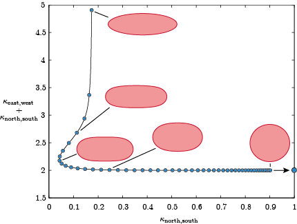
In the context of publication [1] we plot also the cardinal curvatures that has been logged by mat.LogCustom(1,3). Column 2 and 4 in log1.txt contain the curvatures at every timestep. We normalize the curvature by the curvature of the circular interface. The north and east curvature tends to 1, hence the final state in the diagram is (2,1), however we observe that sum of curvatures equal 2 is attained much earlier.
References:
[1] Generic path for droplet relaxation in microfluidic channels, P.-T. Brun, Mathias Nagel, and François Gallaire, Phys. Rev. E 88, 043009