Compile and run
In order to run the first example go into the ulambator folder and type `make tutorial3`. An executable will be created. Type `cd ..` and copy it to a work directory of your choice then type `./tutorial3.o` to execute the program.
You can configure the program with a folder ID, aspect ratio W/2H, shear rate G and droplet radius R: `./tutorial3.o ID W/2H G R`.
Tutorial 3 – Droplet stretching
This tutorial shows interaction of outer boundaries and a liquid interface. Droplet stretching in a cross flow geometry as published in experiments by Ulloa et al. is simulated.
/* Ulambator configuration file Date: 19.12.2014 Version 0.7 */File Header
#include <iostream> #include <stdio.h> #include "../source/matblc1.h" #include "../source/bndblock.h" #include <sys/time.h> #include <time.h> #include <math.h> #include <stdlib.h> int main (int argc, char * const argv[]) { std::cout<<"Welcome to ULAMBATOR++ v0.7\n"; char* savedir; savedir = new char[120]; sprintf(savedir,".");Reading problem parameters
A folder id to number the output folder, the viscosity ratio $\lambda=\mu_{drop}/\mu_{bulk}$, theoretical shear rate G and droplet radius rdrop. The aspect ratio is $200 \mu m$ over $58 \mu m$.
int folderid = 0; double lambda = 0.008; double G = 6.5; double WH = 3.45; int num_elements = 400;The radius is given in micrometers and non-dimensionalized later with the half channel width. Ulloa et al. used two different kind of microchannels, here we configure channel II with a width of $400 \mu m$. The non-dimenseional channel width is 2, thus one unit corresponds to $200\mu m$.
double width = 400.0; double rdrop = 100.0;Reading in data from command line, then non-dimensionalizing the droplet radius.
if (argc>4) { folderid = atoi(argv[1]); WH = atof(argv[2]); G = atof(argv[3]); rdrop = atof(argv[4]); } rdrop = 2*rdrop/width;The theoretical shear rate G is transformed into a inflow velocity: $u = G \cdot W$, where the non-dimensional velocity is $U = \frac{\gamma}{\mu}$. So the non-dimensional inflow rate defines a capillary number $Ca = \frac{\mu\,G\,W}{\gamma}$. The viscosity of the continuous phase is $120 m Pa s$ and the surface tension $48 m Pa m$.
double Ca = G*1e-6*width*120.0/48; std::cout<<"folder:"<<folderid<<" W/2H:"<<WH<<" G:"<<G<<" Rd:"<<rdrop<<"\n";Defining the geometry
A boundary block with two boundries is created.
BndBlock bem(2);Decide to use boundaries or an infinite hyperbolic flow profile without outer boundaries. Without outer boundaries it is faster but requires a correction from the theoretical shear rate in the channel to the shear rate of the infinite flow.
double bcs[] = {Ca, 0.0}; double pos[6]; int no_walls = 0; if (no_walls==1) { std::cout<<"In infinite linear flow\n"; bcs[0] = -Ca/1.1; bem.Elements[0].Init(1, 10, 0); bem.PanelInit(0, 0, 0, 7, bcs, pos); } else { std::cout<<"In a cross channel flow\n";Initiate a boundary with 12 panels and 2200 elements. The final zero sets fixed outer boundaries. Following entries set the panel coordinates and initialize every panel.
bem.Elements[0].Init(12, 2200, 0); pos[0] = -6; pos[1]= 1.0; pos[2]= -6.0; pos[3] = -1.0; bem.PanelInit(0,100, 0, 3, bcs, pos); // an inflow panel pos[0] = -6.0; pos[1]= -1.0; pos[2]= -1.0; pos[3] = -1.0; bem.PanelInit(0,250, 0, 0, bcs, pos); pos[0] = -1.0; pos[1] = -1.0; pos[2] =-1.0; pos[3]= -4.0; bem.PanelInit(0,150, 0, 0, bcs, pos); bcs[0] = 0.0; pos[0] = -1.0; pos[1]= -4.0; pos[2]= 1.0; pos[3] = -4.0; bem.PanelInit(0,100, 0, 2, bcs, pos); // an outflow panel pos[0] = 1.0; pos[1]= -4.0; pos[2]= 1.0; pos[3] = -1.0; bem.PanelInit(0,150, 0, 0, bcs, pos); pos[0] = 1.0; pos[1]= -1.0; pos[2]= 6.0; pos[3] = -1.0; bem.PanelInit(0,250, 0, 0, bcs, pos); bcs[0] = Ca; pos[0] = 6.0; pos[1]= -1.0; pos[2]= 6.0; pos[3] = 1.0; bem.PanelInit(0,100, 0, 3, bcs, pos); // an inflow panel pos[0] = 6.0; pos[1]= 1.0; pos[2]= 1.0; pos[3] = 1.0; bem.PanelInit(0,250, 0, 0, bcs, pos); pos[0] = 1.0; pos[1]= 1.0; pos[2]= 1.0; pos[3] = 4.0; bem.PanelInit(0,150, 0, 0, bcs, pos); bcs[0] = 0.0; pos[0] = 1.0; pos[1]= 4.0; pos[2]= -1.0; pos[3] = 4.0; bem.PanelInit(0,100, 0, 2, bcs, pos); // an outflow panel pos[0] = -1.0; pos[1]= 4.0; pos[2]= -1.0; pos[3] = 1.0; bem.PanelInit(0,150, 0, 0, bcs, pos); pos[0] = -1.0; pos[1]= 1.0; pos[2]= -6.0; pos[3] = 1.0; bem.PanelInit(0,250, 0, 0, bcs, pos); }Initialize the droplet interface, with one panel, with an excess number of elements and a droplet, type 2.
bem.Elements[1].Init(1,2*num_elements,2);The initial position $x=-4, y=10^{-6}$ facilitates the drift from the center position. We initialize boundary 1, num_elements elements, geometry type 2 (a circle), boundary condition type 21 (a droplet) and the geometric specifications pos and boundary values bc (not used).
pos[0] = -4.0; pos[1]= 1e-6; pos[2]= rdrop; pos[3] = 0.0; pos[4] = 1.0; bem.PanelInit(1,num_elements , 2, 21, bcs, pos);Remeshing is activated with standard density according to method 0 (default, homogeneous distribution). The initial area of boundary is saved and maintained.
bem.RemeshOn(2*M_PI*rdrop/num_elements, 0); bem.Elements[1].initialArea = bem.getArea(1);Setting up the matrix and solver properties
The matrix object is created with the geometry object, aspect ratio WH, viscosity ratio lambda and cpaillary number Ca. the capillary number is only passed to the LogMatlab() function and does not influence the simulation.
MatBlC1 mat(&bem, WH, lambda, Ca);Enable writing and prepare log files.
mat.EnableWrite(savedir); char *title; title = new char[120]; if(folderid>0){ sprintf(title,"cordero%d", folderid); mat.SubFolder(title); } sprintf(title,"Machine Time\n"); mat.LogPrepare(0, title); mat.LogPrepare(1, ""); bem.LogTimeStep(0); // Log simulation time (no line break) mat.LogRuntime(0); // Log real time bem.LogCustom(1,2); // to logfile 1, with option 2 mat.LogMatlab(); bem.allWrite();To accelerate the simulation in the presence of outer walls the invariant parts of the matrix can be inverted to allow a Gauss block algorithm to decrease the final matrix size.
mat.PreCondense();Solving the problem by time stepping
Set the timestep deltaT to 0.5 and set 10 iterations between output. An outer iteration loop is performed nnSteps times. A total of nSteps*nnSteps are done and the simulated time is deltaT*nSteps*nnSteps.
double deltaT = 0.25; int nSteps = 20; int nnSteps = 110; mat.setTimeStep(deltaT,nSteps);Integrate in time with a Euler explicit one step scheme. Then log data and write geometry. No field variables output is produced, in this version it is incompatible with PreCondense().
for (int j=0; j<nnSteps; j++) { mat.SolveRK1(); bem.LogTimeStep(0); mat.LogRuntime(0); bem.LogCustom(1, 2); bem.allWrite(); } mat.LogRuntime(0); mat.DisableWrite();End of program
std::cout << "Finished and Exiting\n"; return 0; }Results
The animated geometry is visualized with a small Mathematica program. And shows the displacement and deformation of the droplet. The aspect ratio is W/2H = 3.45, G=18 and R= 0.5.
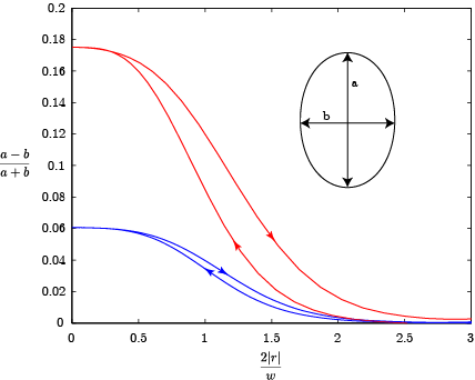
Principle result is the deformation of the droplet in a shear flow. The deformation is defined as the difference of the major and minor axis over the sum of major and minor axis. The blue curve corresponds to the predefined case with G=6.5, R = 100µm (corresponds to Figure 4 (a) in Ulloa et al. [1]). The red curve is for G=18 and R=100µmm, the animation.
References:
[1] Camilo Ulloa, Alberto Ahumada and María Luisa Cordero
Effect of confinement on the deformation of microfluidic drops.
Phys. Rev. E 89, 033004