Compile and run
In order to run the first example go into the ulambator folder and type `make tutorial5`. An executable will be created. Type `cd ..` and copy it to the work directory of tutorial 4 then type `./tutorial5.o` to execute the program.
Alternatively you can adapt the source code of tutorial5.cpp to any other case to provide a posteriori velocity and pressure fields to your simulation.
Tutorial 5 – A posteriori visualization
This tutorial shows how to restart a simulation from a previously saved configuration. Using the reading of a previous configuration we will compute a posteriori the flow field from a simulation that is already finished. The exectuable needs to be copied into the folder where the initial simulation took place.
/* Ulambator configuration file Date: 24.2.2014 Version 0.7 */File Header
#include <iostream> #include <stdio.h> #include "../source/matblc1.h" #include "../source/bndblock.h" #include <sys/time.h> #include <time.h> #include <stdio.h> #include <stdlib.h> #include <math.h> int main (int argc, char * const argv[]) { std::cout<<"Welcome to ULAMBATOR++ v0.7\n"; std::cout<<"Unsteady LAminar Microfluidic Boundary element Algorithm To Obtain Results\n";Reading problem parameters
Working directory, viscosity ratio, capillary number, aspect ratio and a folder id. Since we restart a previous simulation these parameters should match those of the initial simulation.
char* savedir; savedir = new char[120]; sprintf(savedir,"."); double lambda = 0.1; double Ca = 0.001; double RH = 3.0; int folderid = 0;Additionally the radius of the indentation r_hole is provided. Here we set r_hole equal to the channel height.
double r_hole = 1.0/RH; std::cout<<"Configuration folder:"<<folderid<<" R/H:"<<RH<<" Ca:"<<Ca<<"\n"; std::cout<<"lambda:"<<lambda<<" and indentation radius:"<<r_hole<<"\n";Setting up the geometry
Three boundaries, one for the outer flow and two for the droplets.
BndBlock bem = BndBlock(3);Create variables for geometric and boundary value information and initialize the first boundary with 1 panel. The first boundary will be an open domain with constant flow at infinity.
double pos[6]; double bcs[2]; int bnd_id = 0; // first boundary int nb_panels = 1; // number of panels for this boundary int nb_elements=0; // boundary at infinity needs no elements int bnd_type=0; // a fixed wall bem.Elements[bnd_id].Init(nb_panels, nb_elements, bnd_type);Initialize panel 0 of boundary 0 as a boundary at infinity.
int wall_type = 0; // a straight line wall, but unused since there are zero elements int bc_type = 5; // constant flow at infinity bcs[0] = Ca; // velocity at infinity in x-direction bcs[1] = 0.0; // no vertical velocity component bem.PanelInit(bnd_id, nb_elements, wall_type, bc_type, bcs, pos);Initialize boundary 1 as a liquid interface.
bnd_id = 1; nb_elements = 500; bnd_type = 2; bem.Elements[bnd_id].Init(nb_panels,2*nb_elements,bnd_type);Writing is enabled in order to provide a folder from where the data is read. The droplet geometry of droplet 1 is read from a previous timestep, here timestep 0.
bem.EnableWrite(savedir); int timestep = 0; bem.DropRead(bnd_id, timestep);Initialize boundary 2 also as a liquid interface.
bnd_id = 2; nb_elements = 500; bnd_type = 2; bem.Elements[bnd_id].Init(nb_panels,2*nb_elements,bnd_type); bem.DropRead(bnd_id, timestep);Matrix initialization
The matrix object is created and a pointer to the geometry is passed as well as the aspect ratio, viscosity ratio and capillary number.
MatBlC1 mat(&bem, RH, lambda, Ca); mat.EnableWrite(savedir);The model boundary condition for the indentation, option 3, is set up. One parameter is passed, which is the radius of the identation. All other parameters are as the effective depth of the hole are calculated from a model that we presented in an article.
mat.ChoseStatBC(3, r_hole, 0.0);The time step for stabilization is equal to that in the initial simulation.
double deltaT = 1.0;Remeshing is activated not for remeshing purposes but because the approximate inter point distance serves to avoid divergent points near the interface. Points closer to the interface than the inter point distance are not evaluated by integration but are assigned the values obtained on the interface.
bem.RemeshOn(6.28/nb_elements,0);Post–Processing
The Visual output is generated for all 100 times. The droplet geometry is loaded, the unknowns determined and then the flow field constructed.
for(int k=0; k<=100; k++){ bem.DropRead(1, k); bem.DropRead(2, k); mat.Build(deltaT); mat.Solve(); mat.VTKexport(k, 40, -1, 3, -1, 3); }End of the program.
mat.DisableWrite(); std::cout << "Finished and Exiting\n"; return 0; }Results
This post-processing routine fits to the simulation in tutorial 4. After compiling tutorial 5 one copies the executable into the folder, where the results of the simulation from tutorial 4 are saved. One has to make sure that the parameters like capillary number, aspect ratio etc. are the same in both cases. After running the code, the results ulam2dNNNN.vtk and ulamgeoNNNN.vtk can be viewed with ParaView.
The examples below disply the velocity field by vectors and animated with streamlines. The background coloring corresponds to the velocity magnitude.
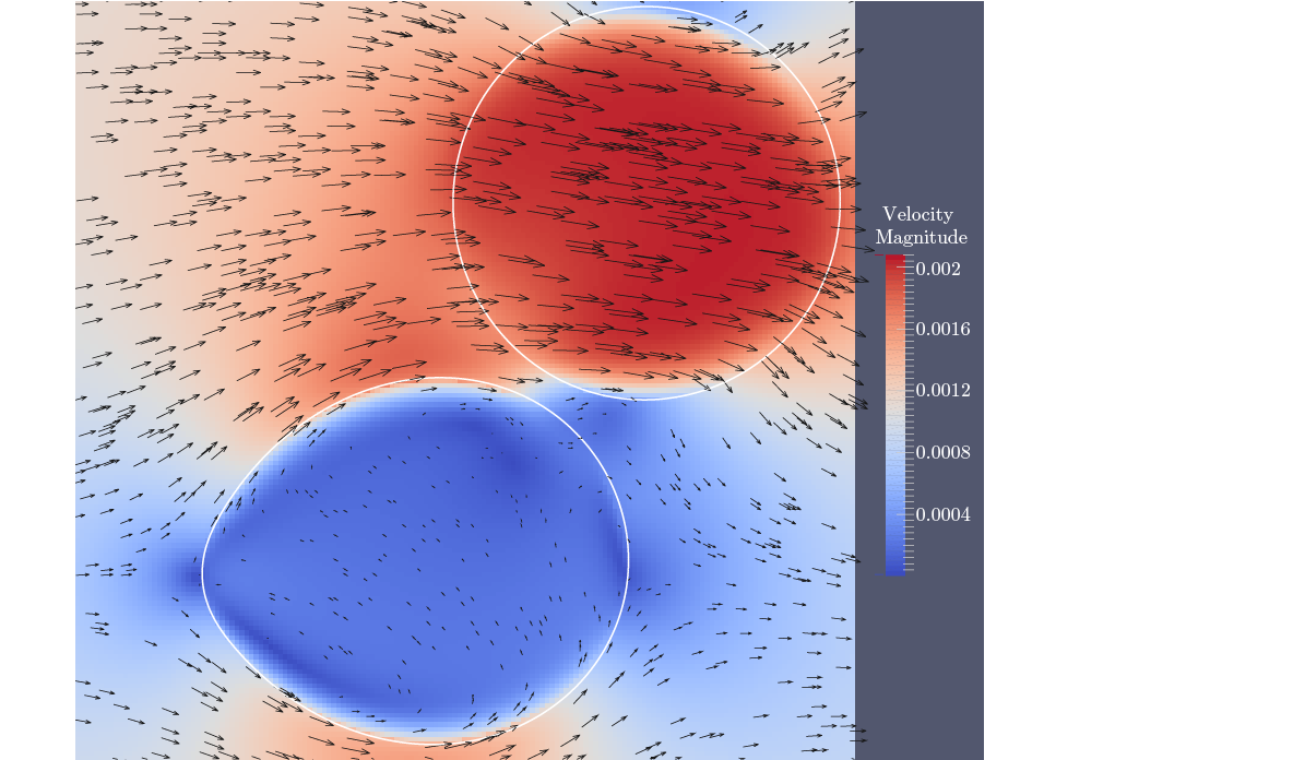
(1) Two droplets in a flow from left to right. The droplet at the bottom is anchored to
an indentation and is at rest, while the upper droplet continues its way.
Aspect ratio R/H=3, viscosity ratio λ =0.1 and capillary number Ca=0.001.